Balance of payments crash course
Why do we do this?
Agenda
Why do we do this?
Current account balance
International investment position
Bilateral international investment position
Net investment income
Why R?
Much more efficient than Excel and much, much more fun
Python just as useful (but I can only teach you R)
Possibilities are endless: For example, all slides for this course are written using R and Quarto
How to get started in R
How to learn R
Start with R for Data Science (2e), by Hadley Wickham, father of the
tidyverse.Datacamp or similar for interactive learning.
Stack Overflow has answers to almost all your questions
AI models got trained on all of the above and are very good at answering coding questions.
DBnomics
- A uniquely helpful platform for official economic data
- Standardized access point to statistical agencies, central banks, and international orgs
- The R package {rdbnomics} makes querying their API easy; downloading data is efficient and reproducible
- This vignette introduces the various options to download data via {rdbnomics}
Install and load packages
Install packages (you need to do this only once; code can be deleted or commented out afterwards):
Load the packages (you need to do this every time you open this script):
Current account balance
Agenda
Why do we do this?
Current account balance
International investment position
Bilateral international investment position
Net investment income
Current account
Exports of goods and services + Receipts of income on UK-owned assets abroad Minus
Imports of goods and services + Payments of income on foreign-owned assets in the United States + Unilateral current transfers
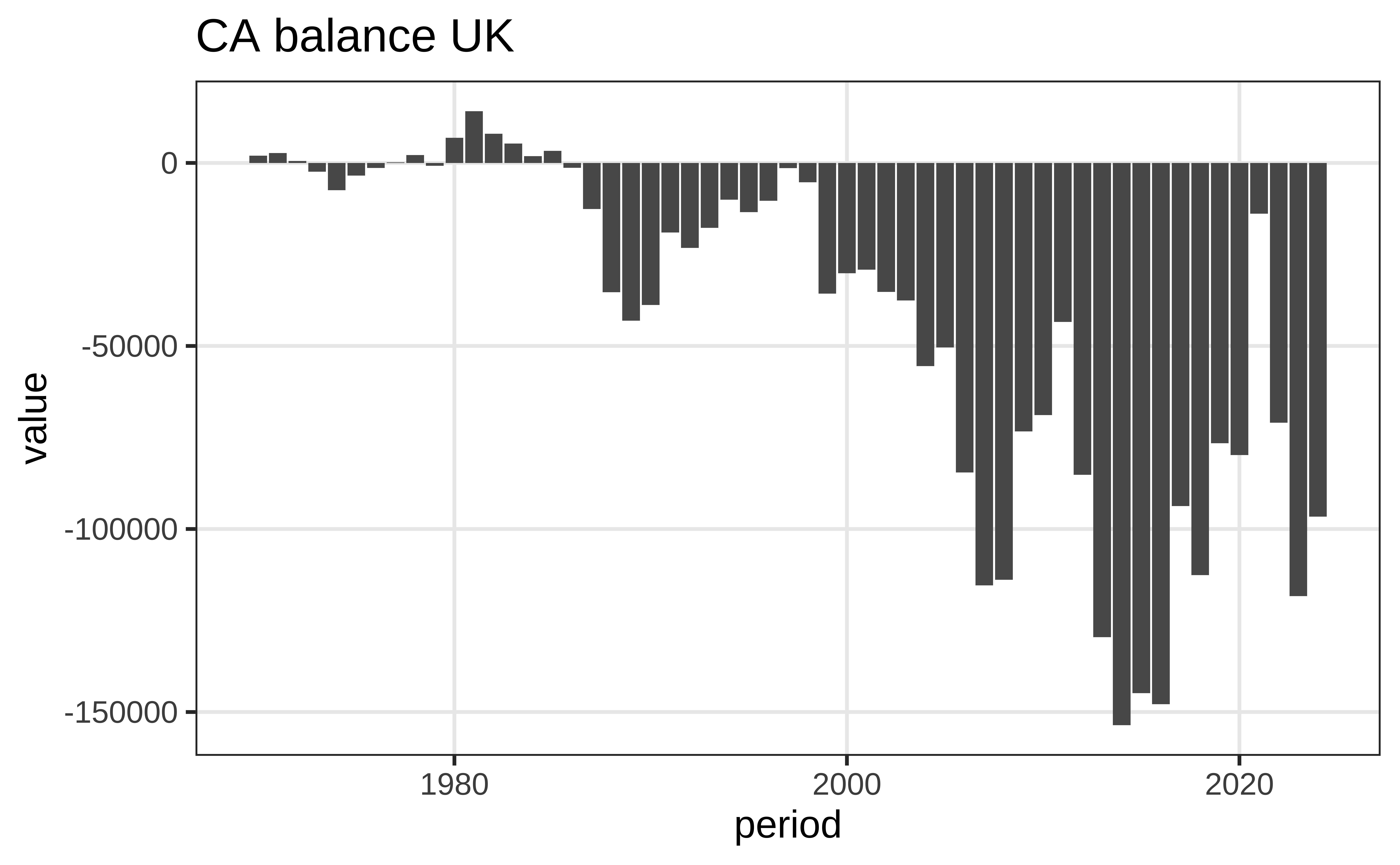
Let’s say we want to download and plot a time series of the UK’s current account balance.
Loading the data
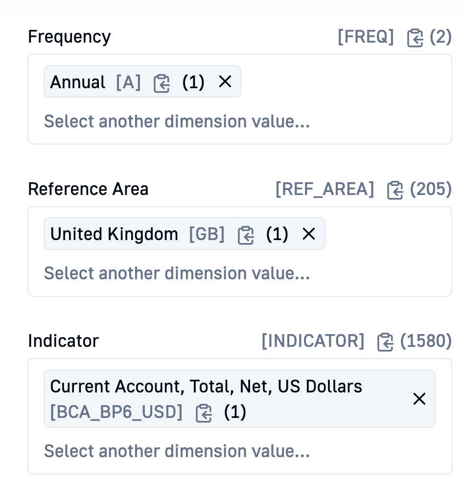
- On DBnomics, select provider (
IMF) and series (BOP) - Use filters to select the UK and, in the field ‘Indicator’, the relevant balance of payments item. Here, we’ll go with
Current Account, Total, Net, US Dollars
Loading the data
- Move to {rdbnomics}. We’ll write our download code using the most efficient method, called ‘masking’ (explained in this vignette):
- Provider:
IMF| Series:BOP - Frequency:
A(annual) - Country:
GB - Indicator:
BCA_BP6_USD
Standard steps
We’ll be working in the Tidyverse: A beginner-friendly ‘dialect’ of R supported by a collection of packages.
- In the Tidyverse, dataframes should be formatted as tibbles. We re-format what {rdbnomics} delivers into a tibble:
Standard steps
- Inspect variable names: Many are standard across DBnomics datasets. Unfortunately, the names are all over the place:
# A tibble: 55 × 5
  Indicator           period     REF_AREA `Reference Area`  value
  <chr>               <date>     <chr>    <chr>             <dbl>
1 Current Account, T… 1970-01-01 GB       United Kingdom    1970.
2 Current Account, T… 1971-01-01 GB       United Kingdom    2717.
3 Current Account, T… 1972-01-01 GB       United Kingdom     533.
4 Current Account, T… 1973-01-01 GB       United Kingdom   -2412.
5 Current Account, T… 1974-01-01 GB       United Kingdom   -7448.
6 Current Account, T… 1975-01-01 GB       United Kingdom   -3465.
# ℹ 49 more rows
Standard steps
clean_namesfrom the {janitor} package let’s us rename variables according to a consistent scheme:
# A tibble: 55 × 5
  indicator             period     ref_area reference_area  value
  <chr>                 <date>     <chr>    <chr>           <dbl>
1 Current Account, Tot… 1970-01-01 GB       United Kingdom  1970.
2 Current Account, Tot… 1971-01-01 GB       United Kingdom  2717.
3 Current Account, Tot… 1972-01-01 GB       United Kingdom   533.
4 Current Account, Tot… 1973-01-01 GB       United Kingdom -2412.
5 Current Account, Tot… 1974-01-01 GB       United Kingdom -7448.
6 Current Account, Tot… 1975-01-01 GB       United Kingdom -3465.
# ℹ 49 more rows
Standard steps
- We use {ggplot2} for plotting. Years go on the x-axis, values on the y-axis. The plot is still empty because we haven’t yet told ggplot what
geomto use to populate it.
Standard steps
- For a bar chart thats
geom_col. And let’s give the plot a title.
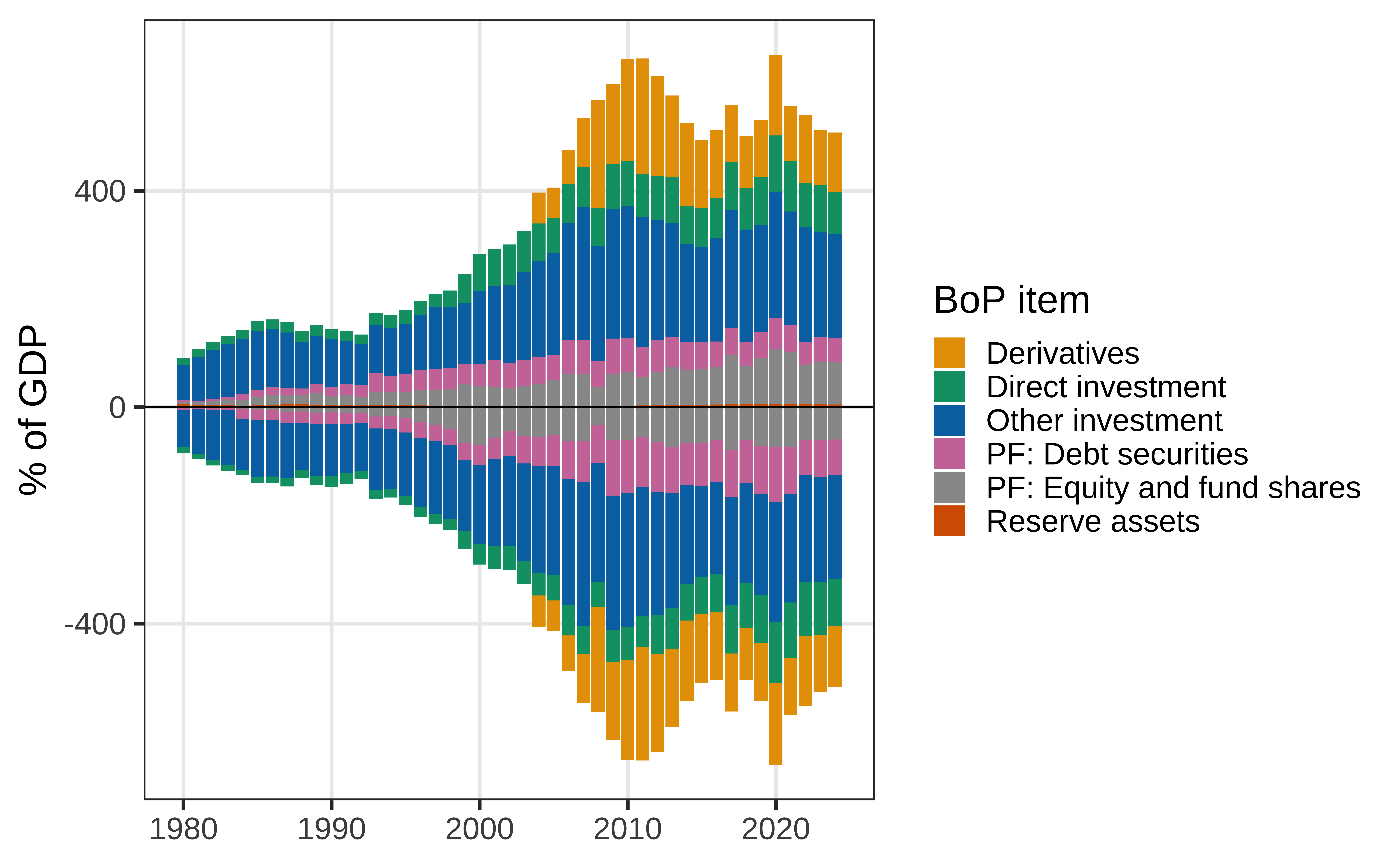
Now that’s nice, but the current account is about trade and investment income flows. What about the UK’s international investment position?
International investment position:
Shows an economy’s stock of external financial assets and liabilities at a particular point
This stock is the result of past external transactions measured according to current market values
Components:
- Credit assets (and debt liabilities)
- Equity assets and liabilities
- Derivatives
- Monetary gold and special drawing rights
International investment position
Agenda
Why do we do this?
Current account balance
International investment position
Bilateral international investment position
Net investment income
Loading the data: IIP & GDP
#Load BOP data using mask method
bop_imf_raw <- rdb("IMF", "BOP", mask = "A.DE+BR+CN+GB+IN+MX.IADF_BP6_USD+IAD_BP6_USD+IAO_BP6_USD+IAPD_BP6_USD+IAPE_BP6_USD+IAR_BP6_USD+ILD_BP6_USD+ILF_BP6_USD+ILO_BP6_USD+ILPD_BP6_USD+ILPE_BP6_USD+ILRRL_NRES_S_BP6_USD")

#Load GDP data using mask method
weo_gdp_raw <- rdb("IMF", "WEO:2024-10", mask = "GER+BRA+CHN+GBR+IND+MEX+USA.NGDPD.us_dollars")

#Convert data frame to tibble format
bop_imf <- as_tibble(bop_imf_raw)
weo_gdp <- as_tibble(weo_gdp_raw)

#Remove rows with missing values
bop_imf <- bop_imf |>
  filter(!is.na(value))

#Clean variable names via 'janitor' package
bop_imf <- clean_names(bop_imf)
weo_gdp <- clean_names(weo_gdp)

#Change confusing country variable name
bop_imf <- bop_imf |>
  rename(country = "reference_area")

weo_gdp <- weo_gdp |>
  rename(country = "weo_country") |>
  rename(gdp_value = "value")

#Select gdp_value
weo_gdp <- weo_gdp |>
  select(period, country, gdp_value)

###Join
bop_imf_gdp <- bop_imf |>
  left_join(weo_gdp)

###Divide by GDP/1000 (GDP is in billion), x100 (for %)
bop_imf_gdp <- bop_imf_gdp |>
  filter(!is.na(gdp_value)) |>
  mutate(value = value/gdp_value/1000*100, .keep = "unused")
To produce the plot on the next slide, we need corresponding assets and liabilities to have identical character values. So let’s create a variable bop_items that fulfils this requirement:
bop_imf_gdp <- bop_imf_gdp |>
  mutate(bop_item = case_when(
    str_detect(indicator, "Derivatives") ~ "Derivatives",
    str_detect(indicator, "Direct Investment") ~ "Direct investment",
    str_detect(indicator, "Other Investment") ~ "Other investment",
    str_detect(indicator, "Debt Securities") ~ "PF: Debt securities",
    str_detect(indicator, "Direct Investment") ~ "Direct investment",
    str_detect(indicator, "Equity") ~ "PF: Equity and fund shares",
    str_detect(indicator, "Reserve Assets") ~ "Reserve assets"))
Since bop_item no longer contains any information about whether we’re looking at an asset or a liability, let’s add a separate asset/liability label variable:
It turns out the indicator column contained two variables—a no-go for tidy data. What we’ve done: We’ve separated the names of the financial instruments from the asset/liability label.
Now we can give a negative sign to all liability values:
Plot the UK’s IIP
Three imbalanced growth models
p <- bop_imf_gdp |>
  filter(ref_area %in% c("BR", "CN", "MX")) |>
  filter(period > "1999-01-01") |>
  filter(!is.na(bop_item)) |>
  ggplot(aes(x = period, y = value, fill = bop_item)) +
  geom_col() +
  geom_hline(yintercept=0) +
  scale_fill_manual(values=okabe_ito()) +
  labs(y = "% of GDP",
       x = NULL,
       fill = "BoP item") +
  facet_wrap(vars(country), scales = "free_y") +
  theme(legend.position = "bottom")
Three imbalanced growth models
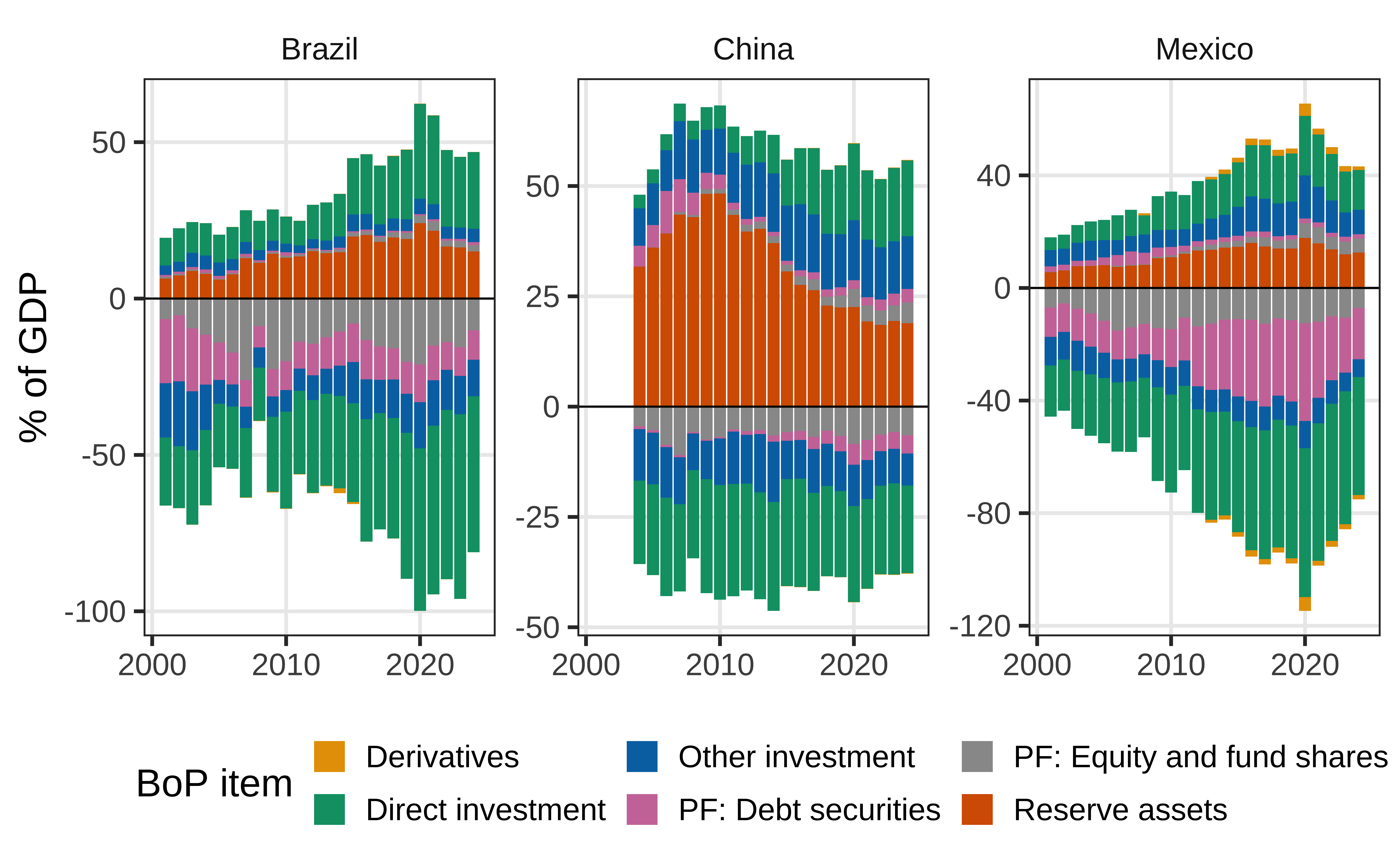
Now that’s nice, but I want to know about my country’s bilateral IIP.
Bilateral international investment position
Agenda
Why do we do this?
Current account balance
International investment position
Bilateral international investment position
Net investment income
Sourcing bilateral IIP data
Bilateral IIP data is not available from the IMF. For European countries, we can go to Eurostat, which luckily is also available via DBnomics.
I started selecting the same BOP items as above for Italy here.
Loading the data
#Eurostat BoP data via rdbnomics package: Assets, liabilities, net-position
#To break down 'Other investment', use FA__O__F2+FA__O__F4+FA__O__F519+FA__O__F81
bop_bil_raw <- rdb("Eurostat", "BOP_IIP6_Q", mask = "Q.MIO_EUR.FA__D__F+FA__F__F7+FA__O__F+FA__P__F3+FA__P__F5.S1.S1.A_LE+L_LE+N_LE.AT+BE+HR+CY+EE+FI+FR+GR+IT+LV+LT+MT+PT+SI+SK+ES+IE+LU+NL+CH+OFFSHO+CN_X_HK+UK+HK+JP+US+IN+RU+BR+WRL_REST.IT")

#Remove missing values
bop_bil <- bop_bil_raw[!is.na(value)]

#Transform data frame into tibble
bop_bil <- as_tibble(bop_bil)

#Clean variable names
bop_bil <- clean_names(bop_bil)

#Convert values to € million to € billion
bop_bil <- bop_bil |>
  mutate(value = value/1000)
Renaming
#Rename BOP items for plotting
bop_bil <- bop_bil |>
  mutate(bop_item = case_when(
    str_detect(balance_of_payments_item, "direct investment") ~ "Direct investment",
    str_detect(balance_of_payments_item, "other investment") ~ "Other",
    str_detect(balance_of_payments_item, "debt securities") ~ "PF: Debt securities",
    str_detect(balance_of_payments_item, "equity") ~ "PF: Equity and fund shares",
str_detect(balance_of_payments_item, "derivatives") ~ "Derivatives"))Further processing
#Select relevant variables
bop_bil <- bop_bil |>
  select(geo, country, country_partner, period, stk_flow, bop_item, value)

#Rename partner countries
bop_bil <- bop_bil |>
  pivot_wider(names_from = country_partner,
              values_from = value) |>
  rename("China" = "China except Hong Kong") |>
  pivot_longer("Austria":"Rest of the world",
               names_to = "country_partner",
               values_to = "value")

#Add negative sign to liabilities
bop_bil <- bop_bil |>
  mutate(value = if_else(stk_flow == "L_LE", -1*value, value))
Plot assets and liabilities for Italy
p <- bop_bil |>
  filter(stk_flow != "N_LE") |>
  filter(!country_partner %in% c("Austria", "Belgium", "Finland",
                                 "Croatia", "Russia", "Portugal",
                                 "Hong Kong", "India",
    "Rest of the world", "Cyprus", "Malta", "Estonia",
    "Slovakia", "Slovenia", "Latvia", "Lithuania")) |>
  ggplot(aes(x = period, y = value, fill = bop_item)) +
  geom_col(position = "stack") +
  scale_x_date(date_minor_breaks = "10 years") +
  scale_fill_manual(values= okabe_ito()) +
  labs(y = "EUR billion",
       x = NULL,
       fill = "BoP item") +
  guides(fill=guide_legend(nrow=2,byrow=TRUE)) +
  facet_wrap(vars(country_partner),
             scales = "free", nrow = 3) +
  theme(legend.position = "bottom")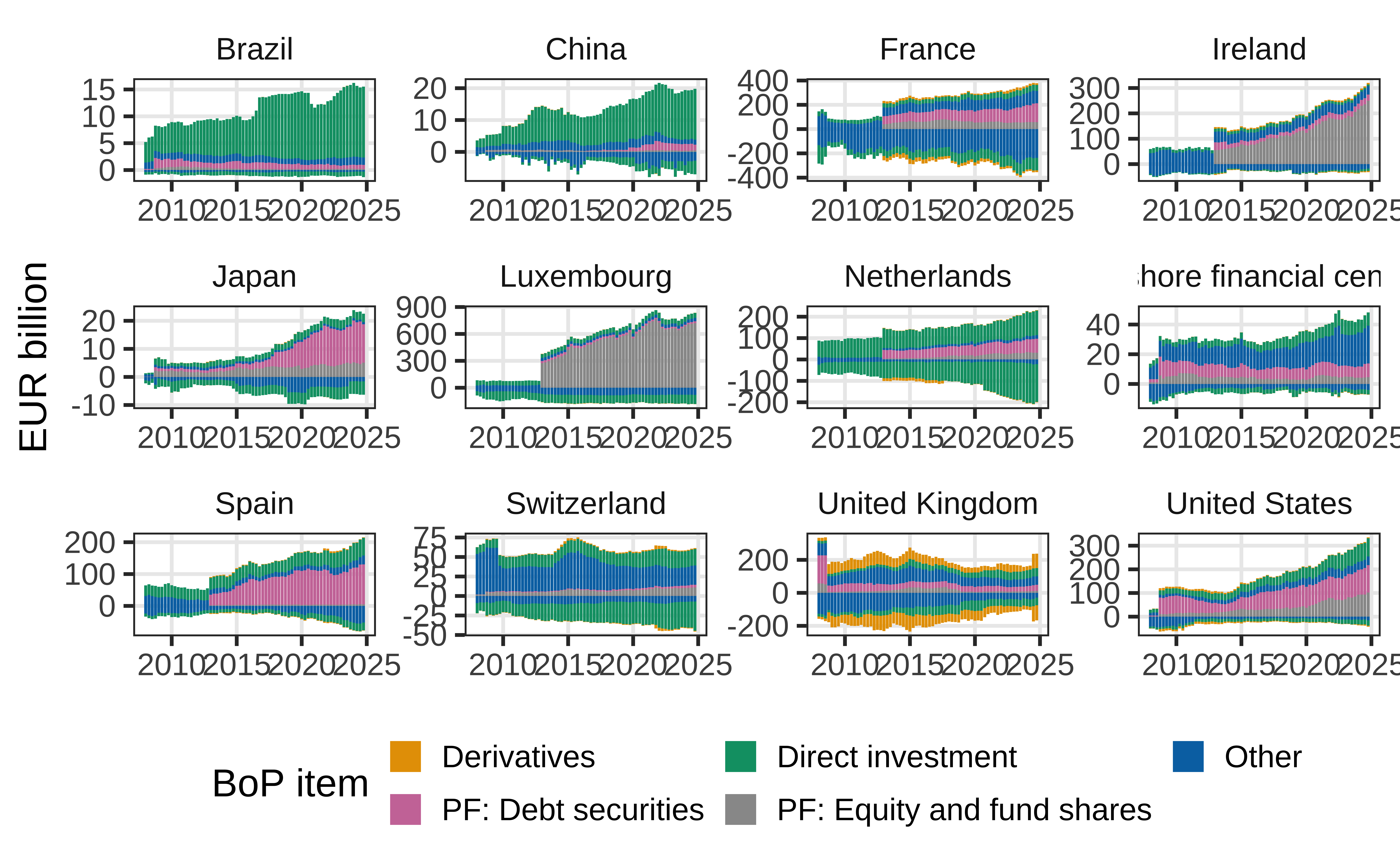
Aggregate countries into groups
bop_bil <- bop_bil |>
  mutate("country_group" = case_when(
    country_partner %in% c("Brazil", "China", "India", "Russia") ~ "BRICs",
    country_partner %in% c("Hong Kong", "Offshore financial centers", "Switzerland") ~ "Financial centers - non-EU",
    country_partner %in% c("Ireland", "Luxembourg", "Netherlands", "Malta", "Cyprus") ~ "Euro area - Financial centers",
    country_partner %in% c("Austria", "Belgium", "Croatia", "Cyprus", "Estonia",
                                           "Finland", "France", "Greece", "Italy", "Latvia", "Lithuania",
                                           "Portugal", "Slovenia", "Slovakia", "Spain") ~ "Euro area - rest",
    .default = country_partner
  ))
Plot assets and liabilities for Italy
p <- bop_bil |>
  filter(stk_flow != "N_LE") |>
  filter(period >= "2008-01-01") |>
  filter(!country_group %in% c("Rest of the world", "Japan")) |>
  group_by(period, country_group, bop_item, stk_flow) |>
  summarise("value" = sum(value, na.rm = TRUE)) |>
  ggplot(aes(x = period, y = value/1000, fill = bop_item)) +
  geom_col(position = "stack") +
  scale_fill_manual(values= okabe_ito()) +
  labs(y = "EUR trillion",
       x = NULL,
       fill = "BoP item") +
  facet_wrap(vars(country_group), scales = "free_x") +
  theme(legend.position = "bottom") +
  guides(fill=guide_legend(nrow=2,byrow=TRUE))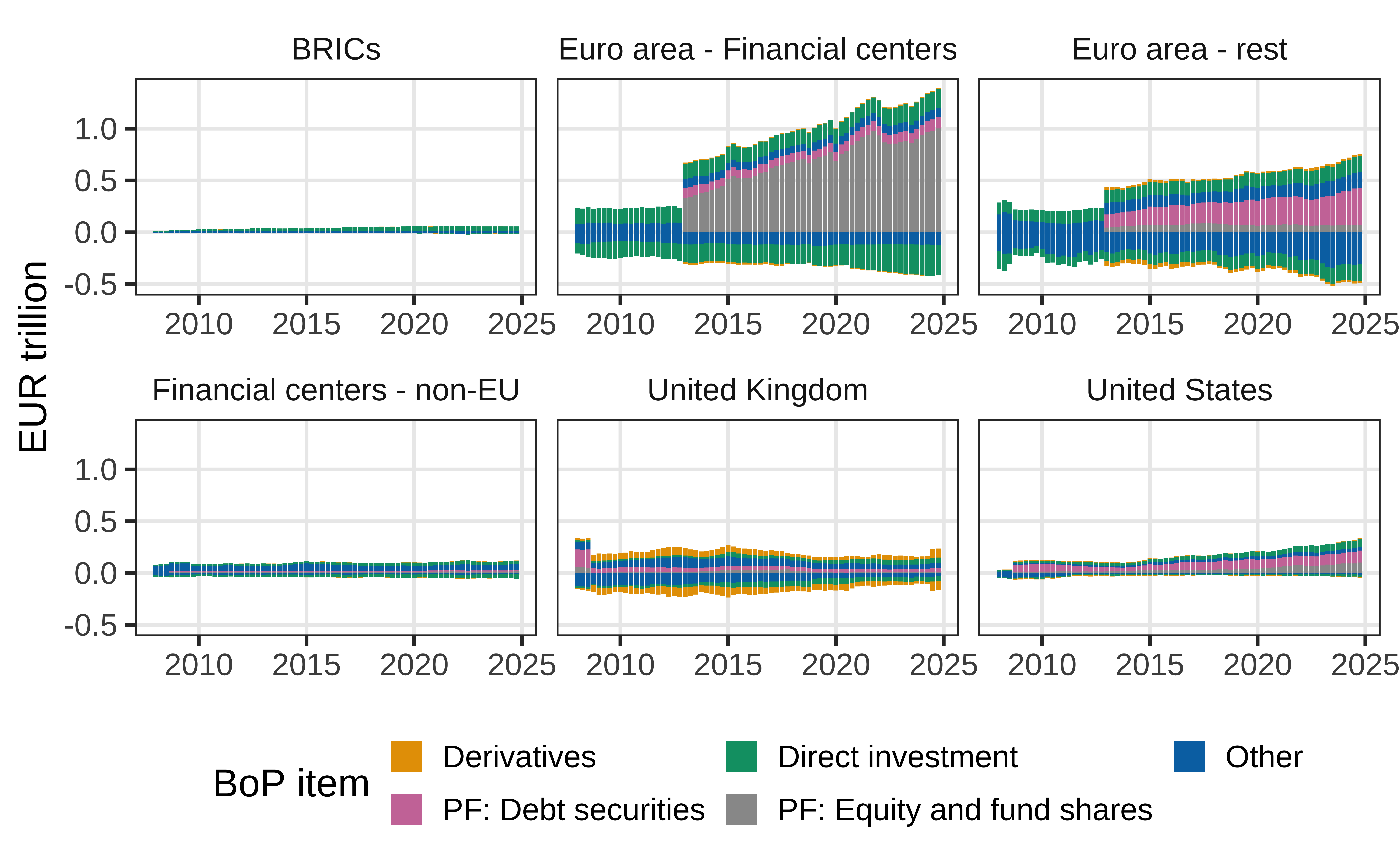
Net investment income
Agenda
Why do we do this?
Current account balance
International investment position
Bilateral international investment position
Net investment income
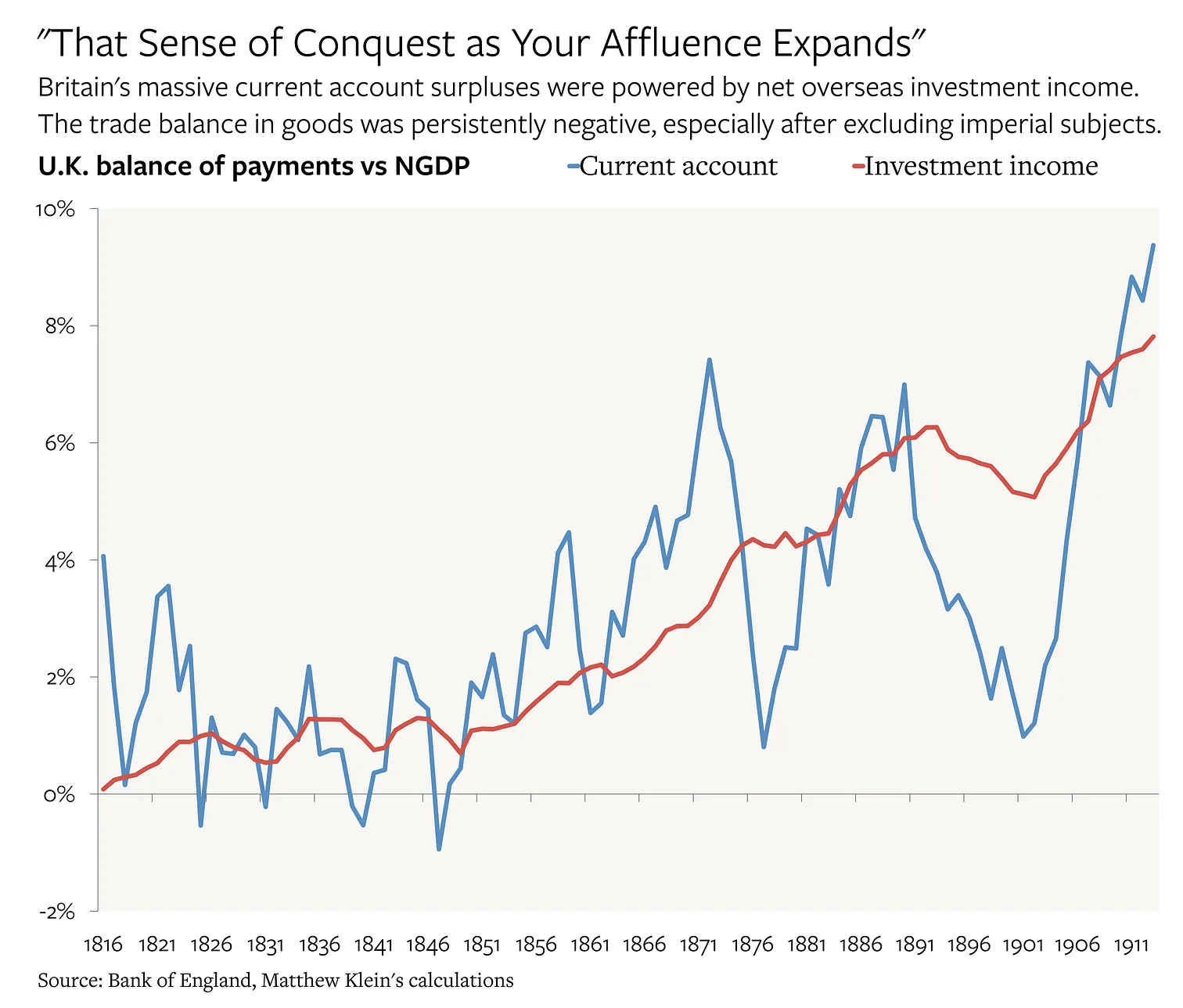
Primacy if investment income
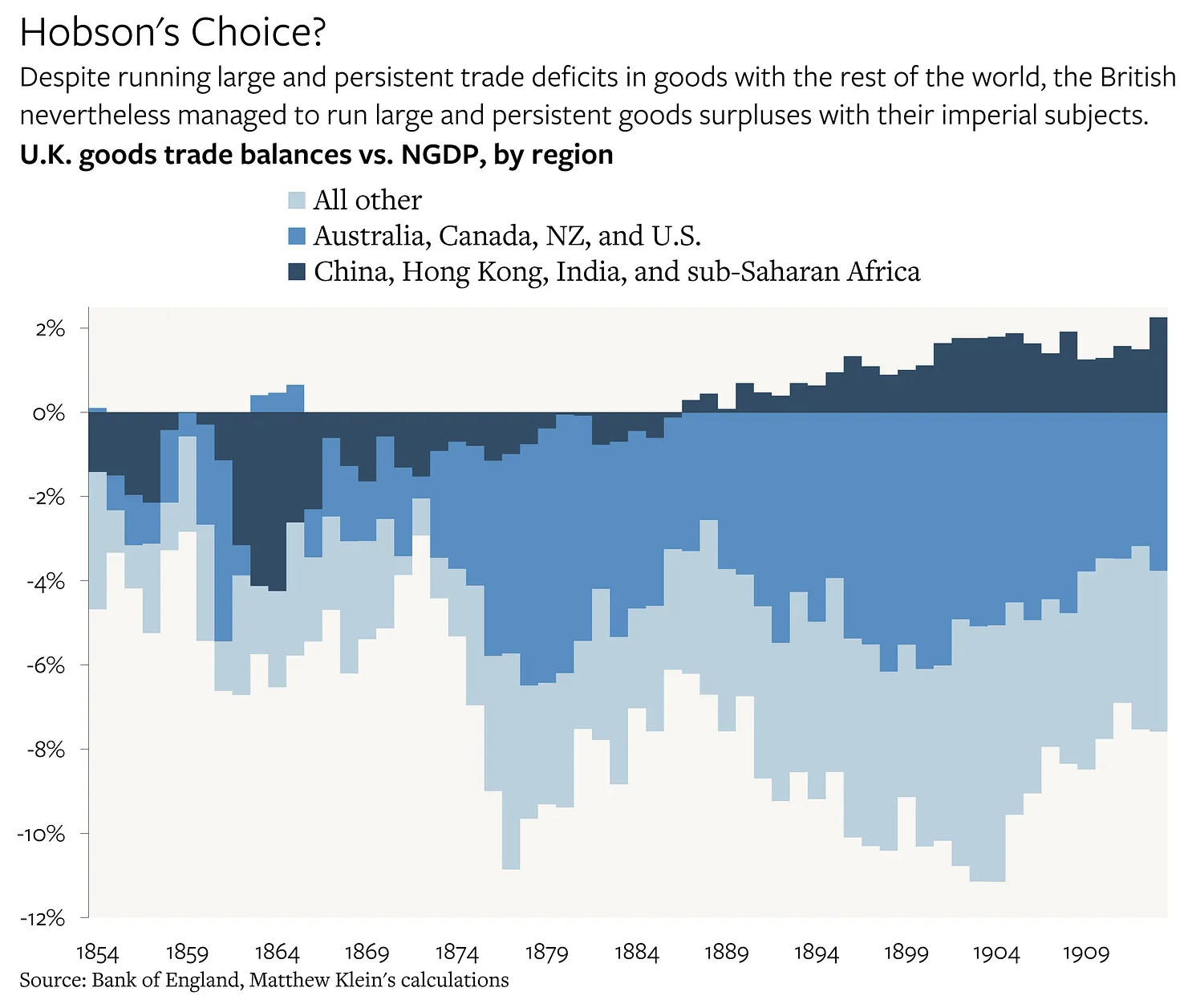
Source: Matthew Klein.
Primacy if investment income
Source: Matthew Klein.
Primacy if investment income
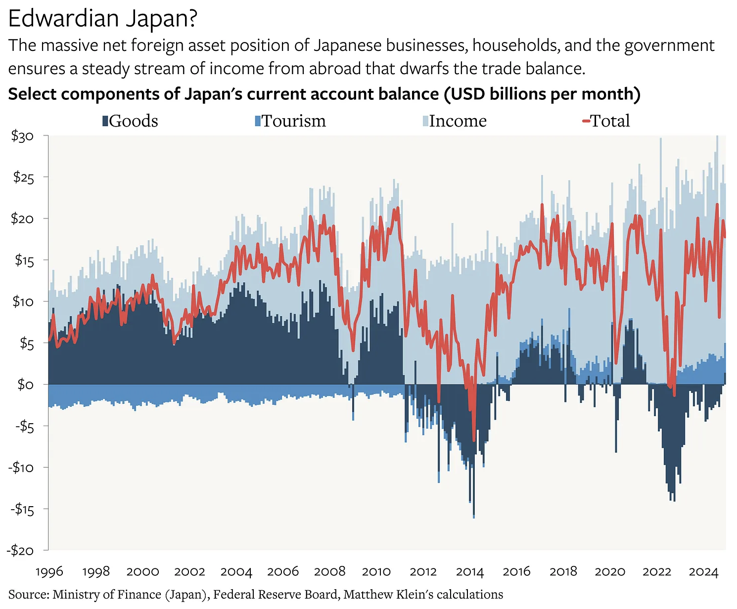
Source: Matthew Klein.
Net investment income
So far, by looking at the IIP, we have been looking at stocks: assets and liabilities
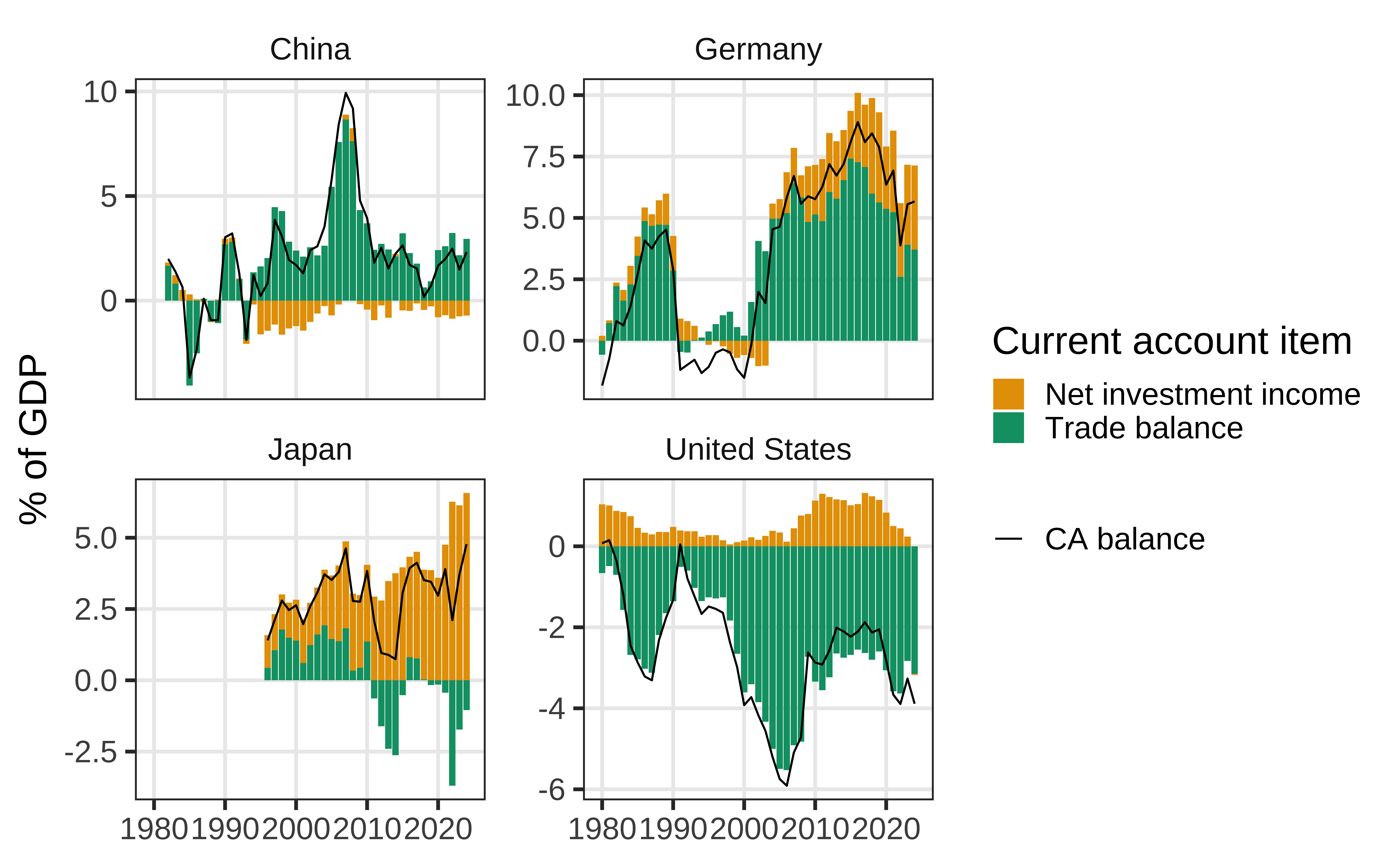
But flows matter. Remember: Current account balance = Trade balance + net earned income
Earned income (as it is called in BoP 7th ed.) or ‘primary income’ (BoP 6th ed.):
- Income associated with the production process includes remuneration of employees, taxes on production and on imports, and subsidies.
- Property income is the income receivable by the owner of a financial asset or the owner of a nonproduced natural resource or another nonproduced nonfinancial asset in return for providing funds to, or putting the nonfinancial assets at the disposal of, anotherinstitutional unit (that is, investment income and rent).
For countries with large IIP stocks, net earned income can easily exceed the trade balance.
Loading and processing the data
- To select the relevant indicators, back to dbnomics for net primary income data and, again, for GDP data
#Load primary income data from IMF
bop_imf_raw <- rdb("IMF", "BOP", mask = "A.DE+JP+US+CN.BCA_BP6_USD+BGS_BP6_USD+BG_BP6_USD+BIP_BP6_USD+BIPCE_BP6_USD+BIPID_BP6_USD+BIPIO_BP6_USD+BIPIPE_BP6_USD+BIPIPI_BP6_USD+BIPO_BP6_USD+BXIPIRI_BP6_USD+BMIP_BP6_USD+BXIP_BP6_USD+BIPI_BP6_USD")

#Load GDP data from IMF
weo_gdp_raw <- rdb("IMF", "WEO:2024-10", mask = "CHN+DEU+JPN+USA.NGDPD.us_dollars")

#Convert data frame to tibble format
bop_imf <- as_tibble(bop_imf_raw)
weo_gdp <- as_tibble(weo_gdp_raw)

#Remove rows with missing values
bop_imf <- bop_imf |>
  filter(!is.na(value))

#Clean variable names via 'janitor' package
bop_imf <- clean_names(bop_imf)
weo_gdp <- clean_names(weo_gdp)

#Change confusing country variable names
bop_imf <- bop_imf |>
  rename(country = "reference_area")

weo_gdp <- weo_gdp |>
  rename(country = "weo_country") |>
  rename(gdp_value = "value")

#Select value
bop_imf <- bop_imf |>
  select(period, country, indicator, value)

#Select gdp_value
weo_gdp <- weo_gdp |>
  select(period, country, gdp_value)

###Join
bop_imf_gdp <- bop_imf |>
  left_join(weo_gdp)

###Divide by GDP*1000 (GDP values are in billion USD) *100
bop_imf_gdp <- bop_imf_gdp |>
  filter(!is.na(gdp_value)) |>
  mutate(value = value/gdp_value/1000*100, .keep = "unused")

#Rename indicators
#Pivot wider
bop_imf_gdp <- bop_imf_gdp |>
  pivot_wider(names_from = indicator, values_from = value)

#Assign new names
names(bop_imf_gdp) <- c("period", "country", "CA balance", "Trade balance",
                        "Trade balance: Goods", "Compensation of employees", "Direct investment", "Other investment",
                        "Portfolio investment: equity", "Portfolio investment: debt",
                        "Net primary income - investment", "Other primary income",
                        "Net investment income", "Total primary income payments", "Total primary income receipts",
                        "Reserve assets")

#Assign negative sign to payments
bop_imf_gdp <- bop_imf_gdp |>
  mutate("Total primary income payments" = -1*`Total primary income payments`)

#Select CA balance, goods and services balance and net primary income
df_ca_disaggregated <- bop_imf_gdp |>
  select(1:4, `Net investment income`) |>
  pivot_longer(4:5, names_to = "ca_component", values_to = "value")

#Pivot longer
ca <- bop_imf_gdp |>
  select(1:5) |>
  pivot_longer(3:5, names_to = "ca_indicator", values_to = "ca_value")

total <- bop_imf_gdp |>
  relocate(c("Net investment income", "Total primary income payments", "Total primary income receipts", "Net primary income - investment"), .after = country) |>
  select(1:3) |>
  pivot_longer(3, names_to = "primary_income_total", values_to = "total_value")

source <- bop_imf_gdp |>
  select(-c("Net investment income", "Total primary income payments", "Total primary income receipts", "Net primary income - investment",
            "CA balance", "Trade balance", "Trade balance: Goods")) |>
  pivot_longer(3:9, names_to = "primary_income_source", values_to = "source_value")

#Join
df_combined <- source |>
  left_join(total) |>
  left_join(ca)
Investment income & trade balance
#Plot CA components
p <- df_ca_disaggregated |>
  ggplot(aes(x = period, y = value, fill = ca_component)) +
  geom_col() +
  geom_line(aes(y = `CA balance`, color = "CA balance")) +
  scale_fill_manual(values = okabe_ito()) +
  scale_color_manual(values = "black") +
  labs(x = NULL,
       y = "% of GDP",
       fill = "Current account item",
       color = NULL) +
  facet_wrap(vars(country), scales = "free_y")
Investment income & trade balance
Political econmomy of finance summer school 2025
